AudioVisual Data in DH
Advances in Digital Music Iconography: Benchmarking the detection of musical instruments in unrestricted, non-photorealistic images from the artistic domain

Introduction: the era of the pixel
The Digital Humanities constitute an intersectional community of praxis, in which the application of computing technologies in various subdisciplines in the Geisteswissenschaften plays a significant role. Surveys of the history of the field 1 have stressed that most of the seminal applications of computing technology were heavily, if not exclusively, text-oriented: due to the hardware and software limitations of the time, analyses of image data (but also audio or video data) remained elusive and out of practical reach until relatively late, certainly at a larger scale. In the past decade, the application of deep neural networks has significantly pushed the state of the art in computer vision, leading to impressive advances in tasks such as image classification or object detection 2 3. Even more recently, improvements in the field of computer vision have started to find practical applications in study domains outside of strict machine learning, such as physics, medicine or even astrology. Supported by this technology’s (at times rather naive) coverage in the popular media, the communis opinio has been eager to herald the advent of the “Era of the Pixel”.
In the Digital Humanities too, the potential of computer vision is nowadays increasingly recognized. A programmatic duet of two recent articles on “distant viewing” in the field’s flagship journal 4 5 leads the way in this respect, emphasizing the privileged role these new methodologies can play in the exploration of large data collections in the Humanities. The present paper too is situated in a multidisciplinary project in which we investigate how modern artificial intelligence can support GLAM institutions (galleries, libraries, archives, and museums) in cataloguing and curating their rapidly expanding digital assets. As a case study, we shall work with non-photorealistic depictions of musical instruments in the artistic domain.
The structure of this paper is as follows. First, we motivate and contextualize our case study of musical instruments from within the scholarly framework of music iconography and computer vision, but also from the more pragmatic context of the research project from which this focus has emerged. We go on to describe the construction and characteristics of an annotated benchmark dataset, the MINERVA dataset, that will be released together with this paper, through which we hope to stimulate further research in this area. Using this benchmark data, we stress-test the available technology for the identification and detection of objects in images and discuss the current limitations of systems. To illustrate the broader relevance of our approach, we apply the trained benchmark system ‘in the wild’, on unseen and out-of-sample heritage data, followed by a quantitative and qualitative evaluation of the results. Finally, we identify what seem to be the most relevant directions for future research.
Motivation
Music iconography
The present paper must be understood against the wider scholarly background of music iconography, a Humanities field of inquiry with a rich, interdisciplinary history in its own right. 6 concisely defined music iconography as a field being “concerned with the study of the visual representation of musical topics. Its primary materials include portraits of performers and composers, illustrations of instruments, occasions of music-making, and the use of musical imagery for purposes of metaphorical or allegorical allusion”. Because of this wide range of topics, at the intersection of art history and musicology 7 8, the field takes pride of its interdisciplinarity.
Music iconography deliberately adopts a “methodological plurality” 7 which is increasingly complemented with digital approaches. A major achievement in this respect has been the establishment (in 1971) and continued expansion and curation of an international digital inventory for musical iconography, the Répertoire International d’Iconographie Musicale (RIDIM). Now publicly available as an online web resource (https://ridim.org/), RIDIM functions as a reference image database, designed to facilitate the efficient yet powerful description and discovery of music-related art works 9. The need for such an international inventory has been acknowledged as early as 1929 and its significant scope facilitates the international study of music-related phenomena and their depiction across the visual arts.
Music iconography has an important tradition of focused studies targeting the deep, interpretive analysis of individual artworks or small collections of them. Such hermeneutic case studies have the advantage of depth, but understandably lack a more panoramic perspective on the phenomena of interest and, for instance, diachronic or synchronic trends and shifts therein. The large-scale, “serial” study of musical instruments as depicted across the visual arts remains a desideratum in the field and has the potential of bringing a macroscopic perspective to historical developments. In the present paper, we explore the feasibility of applying methods from present-day computer vision, in an attempt to scale up current approaches. The primary motivation of this endeavour is that digital music iconography – or “Distant” music iconography, in an analogy to similar developments in literary studies 4 5 – in principle has much to gain from such methods, at least if they are carefully applied and in continuous interaction with experts in the domain. Our focal point is the automated identification and detection of individual musical instruments in unrestricted, digitized materials from the realm of the visual arts.
This scholarly initiative is embedded in the collaborative research project INSIGHT (Intelligent Neural Systems as InteGrated Heritage Tools), which aims to stimulate the application of Artificial Intelligence to the rapidly expanding digital collections of a selection of federal museum clusters in Belgium.10 One important, transcommunal aspect to Belgium’s cultural history relates to music and musical history, with the invention of the saxophone by Adolphe Sax as an iconic example. An additional factor is the presence of the Musical Instruments Museum in the capital (Brussels) that contributed significantly to international research projects in this area (and which is a partner in the INSIGHT project). This contextualization, finally, is also important to understand our specific choice for the topic of musical instruments, as a representative and worthwhile case study on the application of modern machine learning technology in digital heritage studies.
Computer vision
The methodology for the present paper largely derives from machine learning and more specifically computer vision, a field concerned with computational algorithms that can mimic the perceptual abilities of humans and their capacity to construct high-level interpretations from raw visual stimuli 11. In the past decade, this field has gone through a remarkable renaissance, following the emergence of powerful learning techniques based on so-called neural networks. In particular the advent of “convolutional” networks 2 has led to dramatic advances in the state of the art for a number of standard applications, including image classification (“Is this an image of a cat or a dog?”) and object detection (“Draw a bounding box around any cats in this image”). For some of these tasks, modern computer systems have even been shown to rival the performance of humans 12. In spite of the impressive advances in recent computer vision research, it is generally acknowledged that the state of the art is still confronted with a number of major, as yet unsolved, challenges. In this section we highlight four concrete issues that are especially pressing, given the focus of this paper on image collections in the artistic domain. These challenges motivate our work from the point of view of computer vision, rather than art history.
Photo-realism
One major hurdle is that computer vision nowadays strongly gravitates towards so-called photo-realistic material, i.e. digitized or born-digital versions of photographs that do not actively attempt to distort the reality they depict. The best example in this respect is the influential ImageNet dataset 12, that offers highly realistic photographic renderings of everyday concepts drawn from WordNet’s lexical database. While some more recent heritage collections of course abound in such photo-realistic material (e.g. advertisements in historic newspapers), traditional photography does not take us further back in time than the nineteenth century 13. Additionally, the Humanities study many other visual arts that prioritize much less photorealistic representation and focus even on completely ‘fictional’ renderings of (potentially imagined or historical) realities. While there has been some encouraging and worthwhile prior work into the application of computer vision to non-photorealistic depictions, this work is generally more scattered and the results (understandably) less advanced than those reported for the photorealistic domain. Inspiring recent studies in this area include 14 15 16 17.
Data scarcity
It is a well-known limitation that convolutional neural networks require large amounts of manually annotated example data (or training data) in order to perform well. To address this issue, the community has released several public datasets over the years 18 12 19 20 21 which has allowed the successful training of a large set of neural architectures 22 23 24. However, the nature of the images included in these datasets is mostly photo-realistic, also because such images are relatively straightforward to obtain and annotate. These image collections are very different in terms of texture, content and availability from the sort of data that can nowadays be found in the digital heritage domain.
Computer vision researchers interested in the artistic domain have attempted to alleviate the relative dearth of training data by either releasing domain-specific datasets 19 20 or through the application of transfer learning 25, a machine learning paradigm which allows the application of neural networks to domains where training data is scarce. For image classification, for instance, these efforts have indeed greatly contributed to overall feasibility of applying computer vision outside the photo-realistic domain 25. Both approaches, however, have limitations when it comes to the complementary task of object detection. Popular datasets such as the Rijksmuseum collection 19 or the more recent OmniArt dataset 20 do not come with the metadata required for object-detection problems.
With this work, we take one step forward in addressing these limitations. Firstly, the MINERVA dataset that we present below, specifically tackles the problem of object detection within the broader heritage domain of the visual arts, introducing a novel benchmark for researchers working at the intersection of computer vision and art history. Secondly, we present a number of baseline results on the newly introduced dataset. The results are reported for a representative set of common architectures, which were pre-trained on photo-realistic images. This allows us to investigate to what extent these methods can be reused when tested on artistic images.
Irrelevant training categories
Previous studies have demonstrated the feasibility of “pretraining”: with this approach, networks are first trained on (large) photorealistic collections (i.e. the source domain) and then applied downstream (or further fine-tuned) on an out-of-sample target domain, that has much less annotated data available. While generally useful, this approach is still confronted with the problem that the annotation labels or categories attested in the source domain are often of little interest within the target domain (i.e. art history, in the present case). The popular Pascal-VOC dataset 26, for instance, tackles the detection of 20 classes, out of which more than a third constitute different kinds of transportation systems, such as trains, boats, motorcycles and cars. Naturally, these means of transportation are very unlikely to be represented in artworks that date back to the premodern period. The more complex MS-COCO dataset 21 presents similar problems: even though the amount of classes increases to 80, most of the objects which should be detected are again unlikely to be represented within historical works of art, since they correspond to objects which have only been relatively recently invented such as “microwave”, “cell-phone”, “tv-monitor”, “laptop”, or “remote”, and the like. This poses a serious constraint when it comes to the use of pre-trained object-detectors for artistic collections. As with most supervised learning algorithms, models trained on these collections will only perform well on the sort of data on which they have been explicitly trained. To illustrate this model bias, we report some (nonsensical) detections in the first row of images presented in Figure 1a.
Robustness of the models
Popular object detectors such as YOLO 27 and Fast R-CNN 28 have been designed to perform well on the above-mentioned photo-realistic datasets. However, the variance of the samples denoting a specific class within these datasets is usually much smaller when compared to that in artistic collections. As an example, we refer to a number of images representing the person class within the Pascal-VOC dataset: we can observe from the two leftmost images of the bottom row of Figure 1 that the representation of a ‘person’ is overall relatively unambiguous and hardly distorted. As a result, the person class is usually easily detected by e.g. the YOLO architecture. However, we can see that this task already becomes harder when a person has to be detected within a painting (potentially with a highly distorted representation of the humans in the scene). As shown by the two rightmost images of the bottom row (Figure 1b), a YOLO-V3 model does not see most of the persons represented in the paintings and misclassifies them as non-human beings (e.g. “bear”).
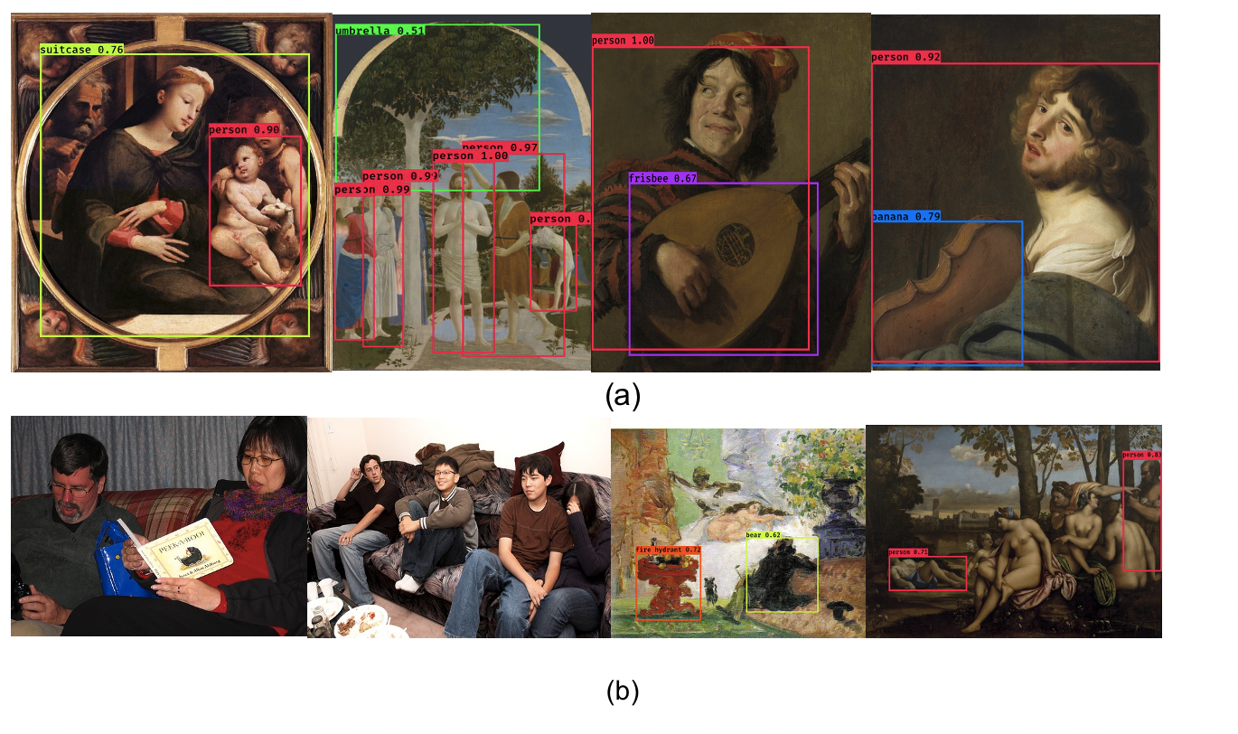
Examples showing the limitations that occur when a standard object detector trained on photo-realistic images is tested in the domain of the visual arts. Figure 1a: Four anecdotal examples showing that the “person” class is usually reasonably detected by the YOLO architecture, although other, non-sensical detections frequently occur. Figure 1b: the two images on the left show that the variation in depiction of people is limited in photorealistic material, in comparison to the artistic representations of people (two examples to the right).
All examples in Figure 1 come from a pretrained YOLO-V3 model 27 which has been originally trained on the COCO dataset 21 and then tested on artworks coming from 19 and 20. The images presented in the first row illustrate that the network is biased towards making detections which are very unlikely to appear in premodern depictions. These detections correspond to the identification of objects such as “suitcase”, “umbrella” or “frisbee” and “banana”. The two last images presented in the second row show that standard models fail to properly recognize a simple class such as person. In fact, they fully fail in detecting most of the persons that are present in the artworks due to these representations being highly different from the persons that are present in the Pascal-VOC dataset (first two images of the second row).
MINERVA: dataset description
In this section, we describe MINERVA, the annotated dataset in the field of object detection that is presented in this work. This novel benchmark dataset will be released jointly with this paper.29 The main task under scrutiny here is the detection of musical instruments in non-photorealistic, unrestricted image collections from the artistic domain. We have named the dataset with the acronym MINERVA, which stands for ‘Musical INstrumEnts Represented in the Visual Arts’, after the Roman goddess of the arts (amongst many other things).
Data Sources
The base data for our annotation effort was assembled in a series of ‘concentric’ collection campaigns, where we started from smaller, but high-quality datasets and gradually expanded into larger, albeit less well curated data sources.
RIDIM: We harvested a collection of high-quality images from the RIDIM database, in those cases where the database entries provided an unambiguous hyperlink to a publicly accessible image. These records were already assigned MIMO codes by a community of domain experts, which provided important support to our in-house annotators (especially during the first experimental rounds of annotations). RMFAB/RMAH: We expanded on the core RIDIM data by including (midrange resolution) images from the digital collections of two federal museums in Brussels: the RMFAB (Royal Museums of Fine Arts of Belgium, Brussels) and the RMAH (Royal Museums of Art and History, Brussels). These images were selected on the basis of previous annotations that suggested they included depictions of musical instruments, although no more specific labels (e.g. MIMO codes) were available for these records at this stage. Copyrighted artworks could not be included for obvious reasons (copyright lasts for 70 years from the death of the creator under Belgian intellectual law). Flickr: To scale up our annotation efforts, finally, we collected a larger dataset of images from the well-known image hosting service ‘Flickr’ (www.flickr.com). We harvested all images from a community-curated collection of depictions of musical instruments in the visual arts pre-dating 1800.30 This third campaign yielded much more data than the former two, but these were more noisy and contained a variety of false positives that had to be manually deleted during the annotation phase.
Our collection efforts were inclusive, and the resulting dataset should be considered as “unrestricted”, covering a variety of periods, genres and materials (although it was not feasible to include more precise metadata about these aspects in the dataset). Note that, exactly because of this highly mixed data origin, the distribution in MINERVA does not give a faithful representation of any kind of historic reality: music iconography gives a highly colored perspective on “popular” instruments in art history and some instruments may not often have been depicted, even though they were popular at the time. Likewise, other instruments are likely to be over-represented in iconography.
Vocabulary
To increase the interoperability of the dataset, individual instruments have been unambiguously identified using their MIMO codes. The MIMO (Musical Instrument Museums Online) initiative is an international consortium, well known for its online database of musical instruments, aggregating data and metadata from multiple heritage institutions 31.32 An important contribution is their development of a uniform metadata documentation standard for the field, including a (multilingual) vocabulary to identify musical instruments in an interoperable manner. The MIMO ontology is hierarchical, meaning that each individual leaf node in their concept tree (e.g. ‘viola’) is a hyponym of a wider instrument category (e.g. ‘viola’ ∈ ‘string instruments’). Table 1 shows examples of annotation labels from this ontology. Our dataset provides a spreadsheet that allows for the easy mapping of individual instruments to their instrument category. Below, we shall report experiments for the more fine-grained and less granular, hypernym versions of the categorization task.
Examples of annotation labels from the MIMO ontology (not all were encountered in MINERVA). Instrument hypernym Stringed instruments Wind instruments Percussion instruments Keyboard instruments Electronic instruments Example instruments Lute, psaltery, fiddle, viola da gamba, cittern Transverse flute, end-blown trumpet, horn, shawm, bagpipe Tambourine, cylindrical drum, frame drum, friction drum, bell Pianoforte, virginal, portative organ, harpsichord, clavichord Electric guitar, synthesizer, theremin, vocoder, mellotron
Annotation process
Using the conventional method of rectangular bounding boxes, we have manually annotated 16,142 musical instruments (of which 172 unique) in a collection of 11,765 images, within the open-source Cytomine software environment 33. Often multiple instruments appeared within the same images and bounding boxes were therefore allowed to overlap. Example annotations and a screenshot of the annotation environment are presented in Figure 2.
The dataset contains artistic objects from diverse periods and of various types, ranging from paintings, sculptures, drawings, to decorative arts, manuscript illuminations and stained-glass windows. Thus, they involve a daunting diversity of media, techniques and modes. Whereas in some cases the images were straightforward to annotate (e.g. an image representing a bell in full frame), several obstacles occurred on a recurrent basis. These obstacles can be linked to three parameters:
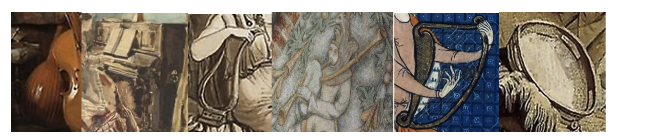
Representation: A challenging aspect was the variety of artistic depiction modes represented in the dataset, ranging from photo-realistic renderings to heavily stylized depictions from specific art-historical movements (e.g. impressionism, pointillism, fauvism, cubism, …) (Figure 3a). Additionally, visibility could be low due to a proportionally small instrument depiction or the profusion of details (Figure 3b). In some instances, the state of the depicted object and its medium made the detection of the instrument difficult, e.g. a damaged medieval tympanon (Figure 3b). Quality: Other, more pragmatic issues arose from the images themselves. Occasionally, the quality of the images was too low to be able to detect the instruments (e.g. low resolution or compression defects) (Figure 3c). A great deal of the images did not meet international quality standards for heritage reproduction photography (uniform and neutral environment and lighting, frontal point of view), which implies that the instruments were even more difficult to detect. Boxes: The use of a rectangular shape for the bounding boxes sometimes has limitations and implied a certain lack of precision, e.g. in the case of a diagonally positioned flute, or in the case of overlapping instruments (Figure 3d). For some instruments which consist of several parts, e.g. a violin and its bow, only the main part (the violin) was annotated.
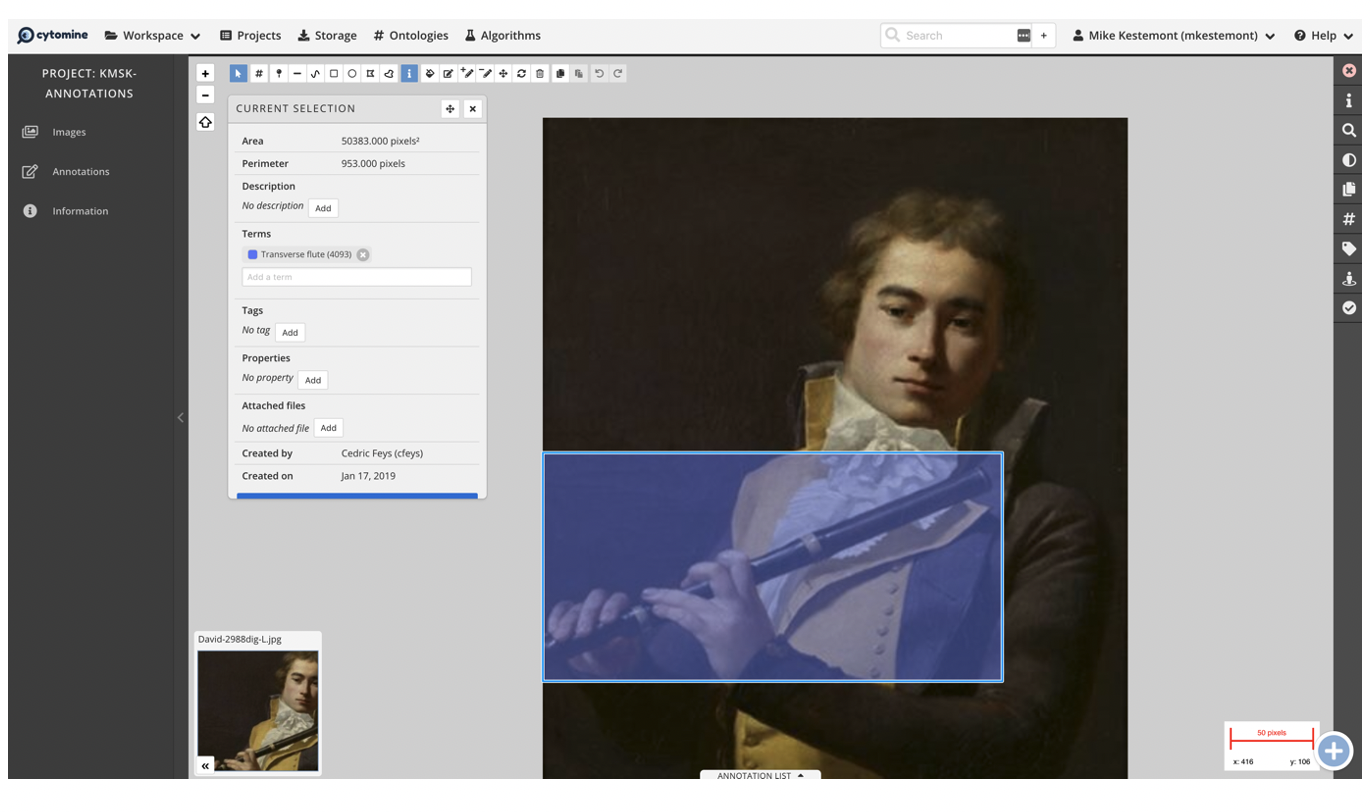
Illustration of the annotation interface in Cytomine [^marée2016].
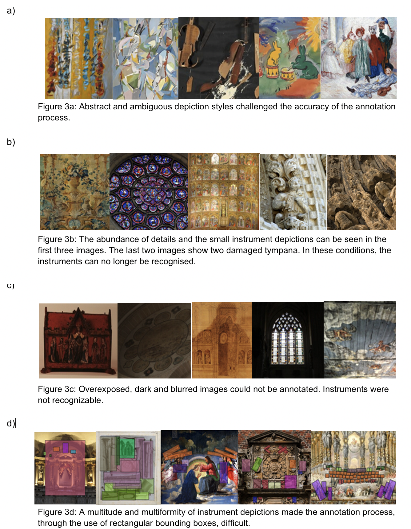
Examples of difficulties encountered when annotating images.
Characteristics
An important share of the annotations which we collected were singletons, i.e. instruments that were only encountered once or twice. Although we release the full dataset, we shall from now on only consider instruments that occurred at least three times that allow for a conventional machine learning setup (with non-overlapping train, validation and test sets, that include at least one instance of each label). Whereas the full MIMO vocabulary covers over 2,000 vocabulary terms for individual instruments, only a fraction of these were attested in the 4,183 images which we use below (overview in Table 1). Note that this table shows a considerable drop in the original number of images that we annotated, because we only included images that (a) actually contained an instrument and (b) images depicting instruments that occurred at least thrice.
93 different instrument categories appear at least thrice in the dataset. A visualization of the heavily skewed distribution of the different instruments can be seen in Figure 4, where each instrument is represented together with its corresponding MIMO code (between parentheses). This distribution exposes two core aspects of this dataset (but also of music iconography in general): (i) its strong Western-European bias, which has been historically acknowledged, and which scholars are actively trying to correct nowadays, but which is a slow process; (ii) the ‘heavy-tail’ distribution associated with cultural data in general; i.e. only a fraction of instruments, such as the lute, harp and violin, are depicted with a high frequency, the rest occurs much more sparsely.
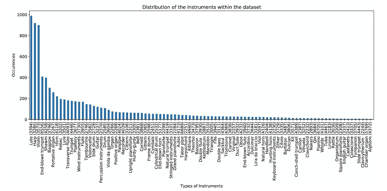
Distribution of the instrument types in the full MINERVA dataset.
Versions and splits
The label imbalance described in the previous paragraph is a significant issue for machine learning methods. We therefore experiment with the data in five versions (that are available from the repository) that correspond to object detection tasks of varying complexity. We start by exploring whether it is possible to just detect the presence of an instrument in the different artworks, without the additional need of also predicting the class of the detected instrument. We refer to this benchmark as single-instrument object detection. We then move to three more challenging tasks in which we also aim at correctly classifying the content of the detected bounding boxes. We include data for this detection task for the top-5, the top-10 and top-20 most frequently occurring instruments, a customary practice in the field. Finally, we also repeat this task for all images, but with the “hypernym” labels of the instrument categories (see Figure 5).
Each version of the dataset comes with its own training, development and testing splits, where we offer the guarantee that at least one of the instrument classes in the task is represented in each of the splits. Additionally, the splits are stratified so that the class distribution is approximately the same in each split. The number of images per split in each version is summarized in Table 2. The hypernym version of the dataset is not reported in this table as it shares the same images and splits as the single-instrument version (they both contain all instruments). We used a standard implementation 34 for a randomized and shuffled split at the level of images and the following, approximate proportions: 1/2 train, 1/4 dev, and 1/4 test. Images may contain multiple instruments, so that the actual number of instruments (as opposed to images) may vary relatively strongly across splits. Distribution of the 5 hypernym categories over the three splits in the MINERVA dataset.
Image and instruments distributions of the training, development and test sets for the four different benchmarks presented in this paper (single instrument, top-5 instruments, top-10 instruments and top-20 instruments). Training-set Dev-set Test-set Total Imag Inst Imag Inst Imag Inst Imag Inst Single inst 1857 4243 1137 2288 1189 2102 4183 8633 Top-5 inst 952 1589 540 852 724 1173 2216 3614 Top-10 inst 1227 2147 680 1127 898 1506 2805 4780 Top-20 inst 1471 2915 860 1543 1047 1838 3378 6296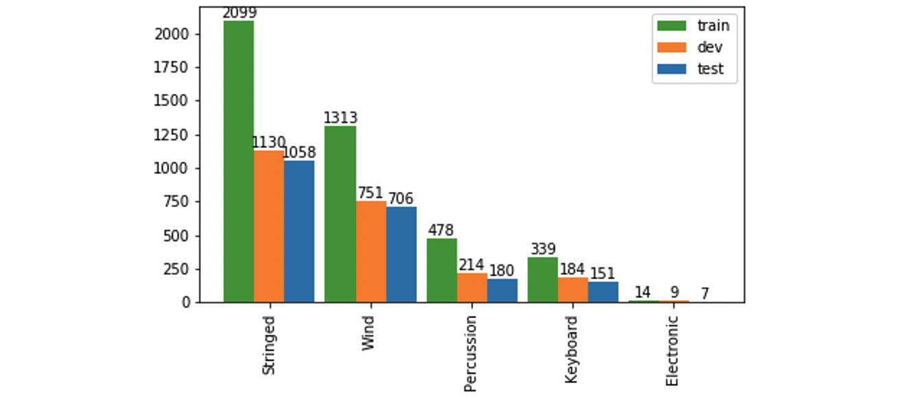
Benchmark experiments
Classification
In the first benchmark experiment, we start by investigating whether convolutional neural networks are able to correctly classify the different instruments that are present in the dataset. That means that we focus on the image classification task and postpone the task of object detection to the next section. To this end, we have extracted the various patches delineated by the bounding boxes in the detection dataset as stand-alone instances. Note, however, that patches from the same images always ended in the same split, to avoid information leakage across the splits. Example patches are shown in Figure 6.
Examples of the patches delineated by the bounding boxes, extracted from MINERVA images for the classification experiment.
Next, we tackled this task as a standard machine-learning classification problem for which we applied a representative selection of established neural network architectures. All of these networks were pretrained on the Rijksmuseum dataset 19, for which the weights are publicly available 25. The tested architectures are: VGG19 24, Inception-V3 23 and ResNet 22. This approach is motivated by previous work 25 which shows that when it comes to the classification images from the domain of cultural heritage, popular neural architectures which have been trained on the large Rijksmuseum collection, can outperform the same kind of architectures that are pre-trained on ImageNet only. In order to maximize the final classification performance, all network parameters get fine-tuned, using the Adam optimizer 35 and minimizing the conventional categorical cross-entropy loss function over mini-batches of 32 samples. Additionally, we applied 3 different learning rates: 0.001, 0.0001, 0.00001. In order to handle the skewed distribution of the classes, we experimented with models including and excluding oversampling. The training regime is interrupted as soon the validation loss does not decrease for five epochs in a row.
In Table 2 and Table 3 we report the results in terms of Accuracy and F1-score for the MINERVA test sets. For the individual instruments, we do so for four versions of the dataset of increasing complexity: the top-5 instruments, top-10 instruments, top-20 instruments and the entire dataset. Analogously we report the scores for a classification experiment where the object detector is trained on the instrument hypernyms as class labels.
Classification results on the MINERVA test set for the three architectures (best results in bold). Top-5 inst Top-10 inst Top-20 inst All inst Hypernyms CNN Acc. F1 Acc. F1 Acc. F1 Acc. F1 Acc. F1 R-Net 68.71 64.10 52.85 41.55 30.73 8.45 26.36 2.08 72.26 52.66 V3 73.66 70.29 55.51 44.77 36.51 19.06 27.02 6.67 75.80 57.03 V19 48.33 35.92 37.52 15.22 33.41 9.87 20.17 1.72 66.41 40.35 Confusion matrix for the classification experiment with ResNet on the MINERVA test set (the top-10 most frequently occurring instruments). Predicted label / Gold label Bagpipe E-b trumpet Harp Horn Lute Lyre Por. organ Rebec Shawm Violin Bagpipe 31 0 10 6 8 1 2 0 7 17 E-b trumpet 4 72 19 2 14 1 3 1 38 21 Harp 8 2 227 1 10 3 11 0 10 19 Horn 7 5 14 9 16 9 1 2 5 14 Lute 6 10 17 6 199 6 5 1 5 42 Lyre 3 0 19 1 13 5 2 0 3 11 Por. organ 3 0 10 1 0 0 57 0 1 4 Rebec 5 2 14 0 9 0 4 7 1 23 Shawm 4 11 25 2 11 2 4 6 40 13 Violin 6 12 29 4 35 4 7 11 6 202
Detection
For the second benchmark experiment we report the results that we have obtained on the four of the five detection benchmarks introduced in the previous section. The way the different instruments are distributed in their respective test sets is visually represented in the first image of each row of Figure 7. For our experiments, we use the popular YOLO-V3 27 architecture which we fully fine-tune during training. To explore the benefits that transfer learning could bring to the artistic domain, we initialize the network with the weights that are obtained after training the model on the MS-COCO dataset 21. The network gets then trained either with the Adam optimizer 35 or RMSprop36 over mini-batches of 8 images.
To assess the performance of the neural network, we follow the same evaluation protocol that characterizes object detection problems in CV 21. Each detected bounding box is compared to the bounding box which has been annotated on the Cytomine platform. We only consider bounding boxes for which the confidence level is ≥ 0.05, following the protocol established in 26. We then compute the “Intersection over Union” (IoU) for measuring how much the detected bounding-boxes differ from the ground-truth ones. To assess whether a prediction can be considered as a “true positive” or a “false positive”, we define two, increasingly restrictive metrics: first, IoU ≥ 10 and, secondly, IoU ≥ 50. This approach is again inspired by 37, where the authors report additional results with an IoU ≥ 10 on their IconArt dataset. Table 5 lists precision, recall and average precision (AP) scores for each detected class of each data version and Figure 7 visually shows the number of true and false positive predictions in all cases. Examples of correct detections are shown in Figure 8. A visual representation of how many instruments should be detected in the testing sets of the four MINERVA benchmarks that are introduced in this paper (first plot of each row). The second and third plots represent the true and false detections that we have obtained with a fully fine-tuned YOLO network. Results are computed with respect to an IoU ≥ 10 and an IoU ≥ 50.
A quantitative analysis of the results obtained on the four localization benchmarks introduced in this work. To distinguish different benchmarks in the table we separate them by a double line. We report the precision, recall and average-precision scores for each detected class. Instrument ≥ IoU Precision Recall AP Single-instrument ≥ 10 Single-instrument ≥ 50 0.63 0.47 0.42 0.31 0.35 0.22 Stringed-Instruments ≥ 10 Stringed-Instruments ≥ 50 0.65 0.53 0.36 0.29 0.28 0.20 Wind-Instruments ≥ 10 Wind-Instruments ≥ 50 0.43 0.32 0.07 0.05 0.04 0.02 Percussion-Instruments ≥ 10 Percussion-Instruments ≥ 50 0.32 0.21 0.04 0.03 0.02 0.01 Keyboard-Instruments ≥ 10 Keyboard-Instruments ≥ 50 0.61 0.45 0.11 0.08 0.07 0.04 Electronic-Instruments ≥ 10 Electronic-Instruments ≥ 50 - - - - - - Harp ≥ 10 Harp ≥ 50 0.68 0.60 0.62 0.54 0.55 0.46 Lute ≥ 10 Lute ≥ 50 0.57 0.47 0.43 0.35 0.36 0.26 Violin ≥ 10 Violin ≥ 50 0.37 0.26 0.22 0.16 0.12 0.07 Shawm ≥ 10 Shawm ≥ 50 0.13 0.08 0.04 0.02 0.01 0.00 End-blown trumpet ≥ 10 End-blown trumpet ≥ 50 0.28 0.24 0.04 0.03 0.01 0.01 Harp ≥ 10 Harp ≥ 50 0.62 0.56 0.56 0.51 0.46 0.39 Lute ≥ 10 Lute ≥ 50 0.55 0.47 0.42 0.36 0.33 0.25 Violin ≥ 10 Violin ≥ 50 0.26 0.20 0.19 0.14 0.06 0.04 Shawm ≥ 10 Shawm ≥ 50 0.17 0.17 0.03 0.01 0.00 0.00 End-blown trumpet ≥ 10 End-blown trumpet ≥ 50 0.67 0.17 0.02 0.03 0.01 0.00 Bagpipe ≥ 10 Bagpipe ≥ 50 0 0 0 0 0 0 Portative-Organ ≥ 10 Portative-Organ ≥ 50 0.24 0.24 0.13 0.13 0.06 0.06 Horn ≥ 10 Horn ≥ 50 0 0 0 0 0 0 Rebec ≥ 10 Rebec ≥ 50 - - - - - - Lyre ≥ 10 Lyre ≥ 50 - - - - – -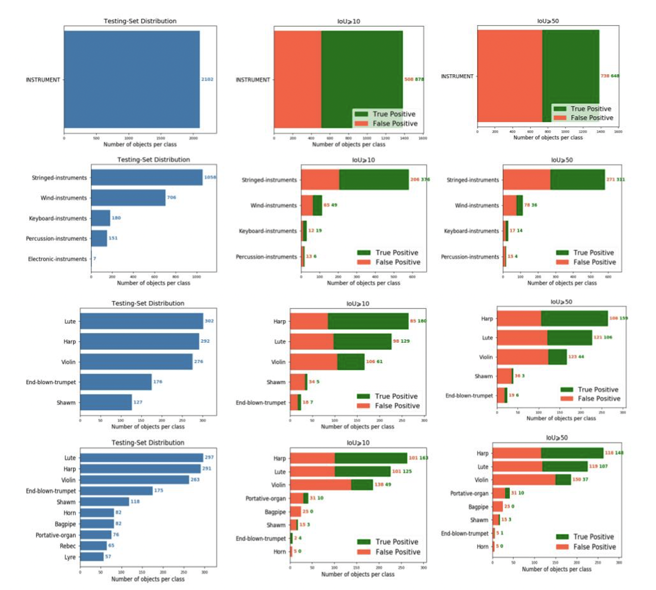
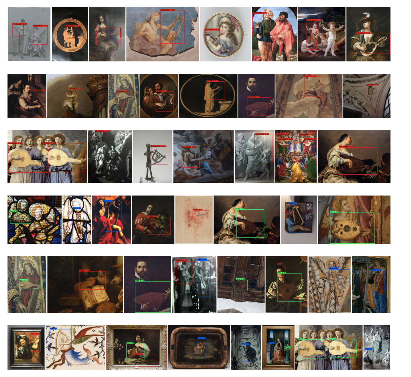
Sample visualizations of the detections obtained on the MINERVA test set for a fully fine-tuned YOLO architecture. The first three rows report the detection of any kind of instrument within the images (single-instrument task), while the last three rows also report the correct classification of the detected bounding boxes.
Additional experiments
As an additional stress-test, we have applied a trained object detector to two external data sets, in order to assess how valid and performant our approach is when applied “in the wild”. We have considered two out-of-sample datasets:
- RMFAB/RMAH: 428 out-of-sample images from the digital assets of both museum collections that are not included in the annotated material (and which are thus not included the train and validation material of the applied detector), because the available metadata did not explicitly specify that they contained depictions of musical instruments. (This collection cannot be shared due to copyright restrictions.)
- IconArt: a generic collection of 6,528 artistic images, collected from the community-curated platform WikiArt: Visual Art Encyclopedia (https://www.wikiart.org/). The IconArt subcollection was previously redistributed by 37: https://wsoda.telecom-paristech.fr/downloads/dataset/.
Note that both external datasets differ in crucial aspects: RMFAB/RMAH can be considered “out-of-sample”, but “in-collection”, in the sense that these images derive from the same digital collections as many of the images represented in MINERVA. Additionally, we can expect extremely low detection rates for this dataset, because the presence of musical instruments will already have been flagged in a large majority of cases by the museum’s staff. Thus, the application of RMFAB/RMAH should be viewed as a rather conservative stress test or sanity check, mainly checking for images that might have been missed by annotators in the past. The IconArt dataset is “out-of-sample” and “out-of-collection”, in the sense that these images derive from a variety of other sources. It is therefore fully unrestricted, and this test can be considered a curiosity-driven validation of the method “in the wild”. Importantly, IconArt was not collected with specific attention for musical instruments, so here too, we can anticipate a rather low detection rate (since many works of art simply do not feature any instruments). For all these reasons, we only evaluate the results on these external datasets in terms of precision (as recall is much less meaningful in this context).
Following these differences, we have applied the single-instrument detector to the RMFAB/RMAH data and the hypernym detector to IconArt. Keeping an eye on the feasibility of the manual inspection, we have limited the number of instances returned by only allowing detections with a confidence score ≥ 0.20 (which is a rather generous threshold). Next, the results have then been evaluated in terms of precision, i.e. the number of returned image regions that actually represent musical instruments. The results are presented in Table 6. Figure 10 showcases a number of cherry-picked successful examples of detections from the out-of-collection IconArt images.
Quantitative evaluation of the method on two out-of-sample datasets in terms of precision, restricted to detections with a confidence score ≥ 0.20. Collection Total images Detections True positives RMFAB/RMAH 428 162 6 IconArt 6528 118 42
Discussion
Skewed results
First and foremost, we can observe that the scores obtained across all benchmarks are generally much lower than those reported for other datasets in computer vision (outside of the strict artistic domain). This drop in performance was to be expected and can be attributed to both the smaller size of the training data and the higher variance in the representation spectrum of musical instruments (across periods, materials, modes and, artists). Secondly, one can observe large fluctuations in the identifiability and detectability of individual instrument categories across both tasks. Not all of the fluctuations are easy to account for.
We first consider the classification results. The confusion matrix reported in Table 4 clearly shows that the classes representing the top-4 of instruments (harp, lute, violin, and portative organ) can be learned rather successfully, but that the performance rapidly breaks down for instrument categories at lower frequency ranks. Thus, while the accuracies for the top-5 experiments are relatively satisfying, especially in terms of accuracy (V3: acc=73.66; F1=70.29 ), the performance rapidly degrades for the more difficult setups. The results for the “all” classification experiment, where every instrument category is included no matter its frequency, are nothing less than dramatic (V3: acc=27.02; F1=6.67 ) and call for in-depth further research. The significant divergence between accuracy scores and F1 scores demonstrate that class imbalance is thus another aspect in which MINERVA presents a more challenging benchmark than its photorealistic counterparts.
The skewness of the class distribution in MINERVA is representative of the long-tail distribution that we commonly encounter in cultural data. This imbalance is somewhat alleviated in the hypernym setup, where the labels are of course much better distributed over a much smaller number of classes ( n=5 ). The general feasibility of this specific task is demonstrated by the encouraging scores that can be reported for the Inception-V3 architecture on this task ( acc=75.80; F1=57.03 ). Note, additionally, that the “Electronic instruments” hypernym is included for completeness in this task, although the label is very infrequent and inevitably pulls down the (macro-averaged) F1-score in this respect. Overall, we notice than the Inception-V3 architecture yields the highest performance on average for the classification task.
Similar trends can be observed for the musical instrument detection task. First of all, we should emphasize the encouraging scores for the “single-instrument” detection task that simply aims to detect musical instruments (no matter their type). Here, a relatively high precision score is obtained ( prec=0.63 for IoU ≥ 10 ), which seems on par with comparable object categories for modern photo-realistic collections 28. Thus, this algorithm might not be fully apt at retrieving every single instrument from an unseen collection, but when it detects an instrument, we can be relatively sure that the detection deserves further inspection by a domain expert. Equally heartening scores are evident for most of the instrument hypernyms (with the notable exception of the under-represented “Electronic instruments” hypernym). While these detection tasks are of course relatively coarse, this observation nevertheless entails that this sort of detection technology can already find useful applications in the field (see below).
When making our way down the frequency list in Table 5, we again observe how the results break down dramatically for less common instrument categories. The fact that an over-represented category like harps can be reasonably well detected ( AP(IoU ≥ 10)=0.55; AP(IoU ≥ 50)=0.46 ), should not lead the attention away from the fact that a state of the art object detector, such as YOLO, fails miserably at detecting a number of iconographically highly salient instruments, such as lyres and end-blown trumpets. At this stage, it is unclear whether this is caused by mere class imbalance or by the higher variance in the iconographic depiction of specific instruments. Bagpipes, for instance, occur frequently across images in MINERVA but might display much more depiction variance than, for instance, a harp.
Saliency maps
The results from the previous question call into question which visual properties the neural networks find useful to exploit in the identification of instruments. Importantly, the characteristic features exploited by a machine learning algorithm need not coincide with the properties that are judged most relevant by human experts and the comparison of both types of relevance judgements is worthwhile. In this section, we therefore perform model criticism or “network introspection” on the basis of the so-called “saliency maps” that can be extracted from a trained model 38. These saliency maps make visible to which regions in the original image the network paid most attention to, before arriving at its final classification decision. All examples discussed below come from the experiments on the hypernym dataset for the VGG19 network. Figure 9 shows a series of manually selected, insightful examples, including the original image (as inputted into the network after preprocessing), as well as the saliency map obtained for it. We limit these examples to the representative hypernyms ‘Stringed instruments’ and ‘Wind instruments.’
The maps in Figure 9 vividly illustrate that the network focuses on two broad types of regions: properties of the instruments itself (which was expected) but also the immediate context of the instruments, and more specifically the way they are operated, handled or presented by people, c.q. musicians. The characteristics of the salient regions in the examples in Figure 9 could be described as:
Stringed instruments:
(a) Focus on the neck of the stringed instrument, as well as the characteristic presence of tuning pins at the end of the neck; (b) Sensitive to the presence of stretched fingers in an unnatural position; (c) Typical conic shape of a lyre, with outward pointing ends connected by a bridge;
Wind instruments:
(d) Symmetric presence of tone holes in the areophone; (e) Elongated, cylindric shape of the main body of the areophone with wider end; (f) Mirrored placement of fingers and hands (close to one another).
These characteristics strongly suggest that the way an instrument is handled (i.e. its immediate iconographic neighborhood) is potentially of equal importance as the shape of the actual instrument, an insight that we will further expand on below.
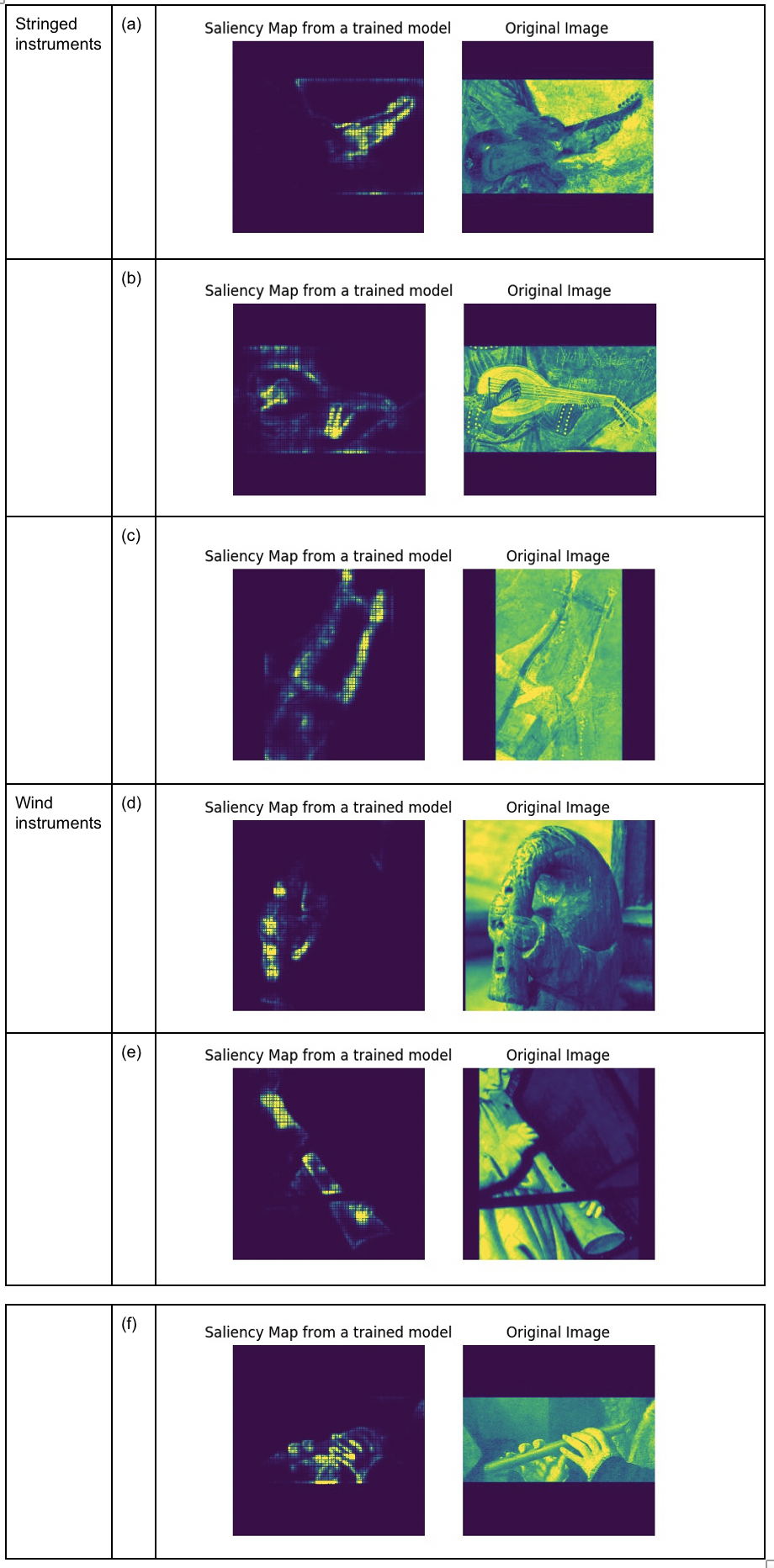
Saliency maps for several stringed (subfigures (a) to (c)) and wind (subfigures (d) to (f)) instruments.
Error analysis: false positives
In this section, we offer a qualitative discussion of the false positives from the out-of-sample tests reported in the previous section, i.e. instances where the detectors erroneously thought to have detected an instrument. This eagerness is a known problem of object detectors: a system that is trained to recognize “sheep” will be inclined to see “sheep” everywhere. Anecdotally, people have noted how misleading contextual cues can indeed be a confounding factor in image analysis. One blog post for instances noted how a major image labeling service tagged photographs of green fields with the “sheep” label, although no sheep whatsoever were present in the images.39 Eagerness-to-detect or over-association is therefore a clear first shortcoming of this method when applied in the wild, mainly because it was only trained in images that actually contain musical instruments. Interestingly, the false positives come in clusters that shed an interesting light on this issue. Below we list a representative number of error clusters:
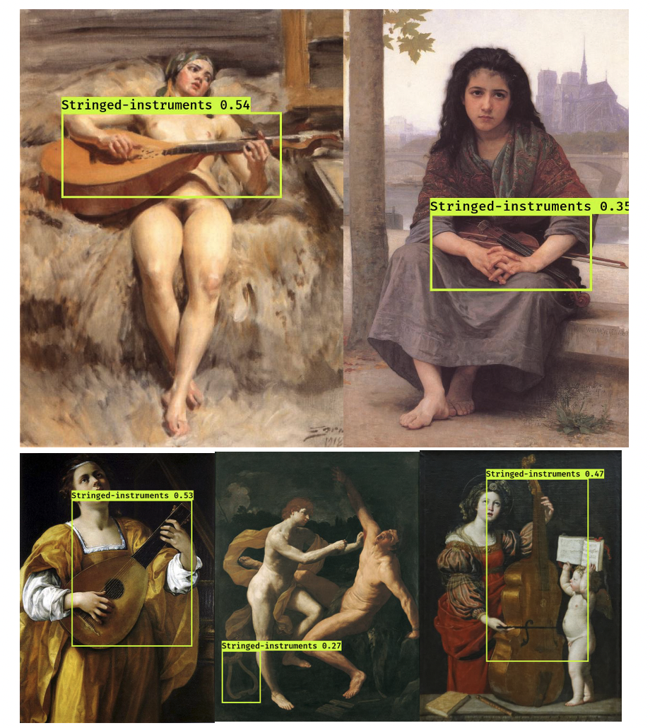
Examples of successful detections in IconArt for “stringed instruments”.
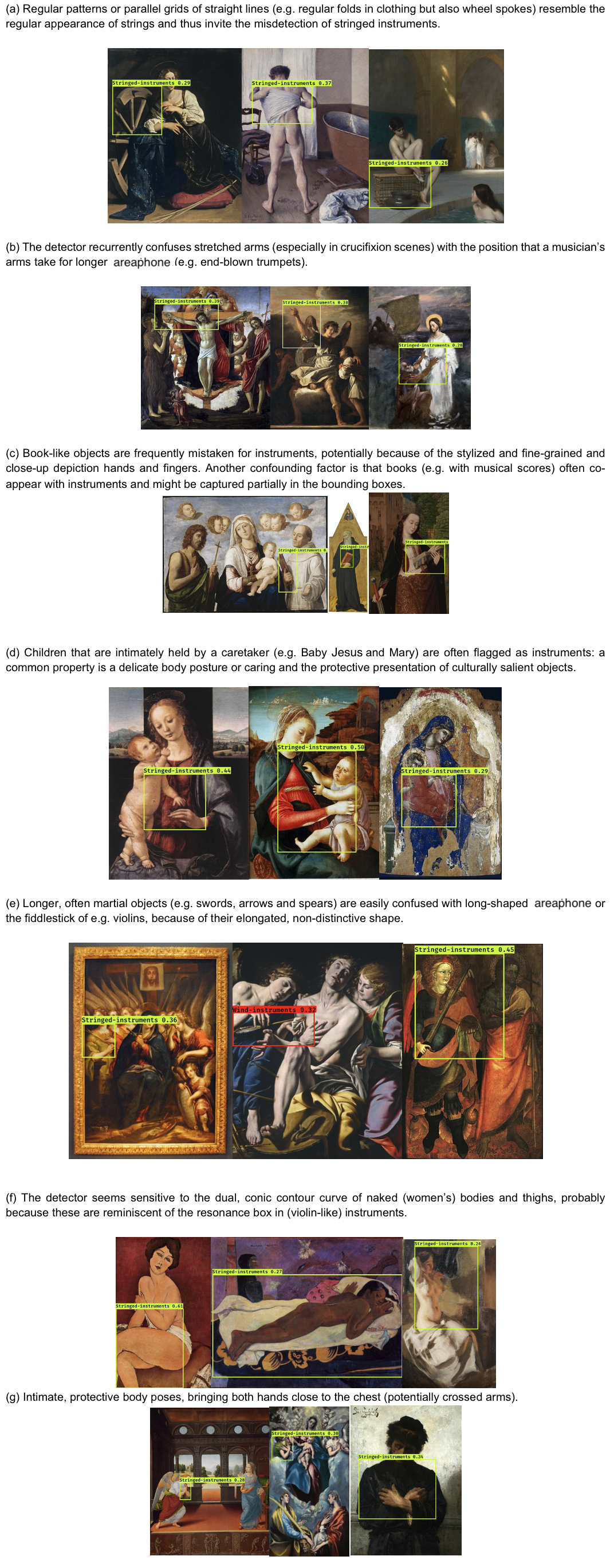
Anecdotal examples of false positive detection, divided in 7 interpretive clusters (numbered a-g).
The above categorization illustrates that the false positives are rather insightful, mainly because the absence of an instrument highlights the contextual clues that are at work. Of particular relevance is the observation that the iconography surrounding children closely resembles that of instruments. This seems related to the intimate and caring body language of both the caretakers and musicians in such compositions. The immediate iconographic neighborhood of children clearly reminds the detector of the delicacy and reverence with which instruments are portrayed and presented in historical artworks. This delicacy and intimacy in body language can be specifically related to the foregrounding of fingers, the prominent portrayal of which invariably triggers the detector, also in the absence of children. Some of these phenomena invite closer inspection by domain experts in music iconography and suggest that serial or panoramic analyses are a worthwhile endeavour in this field, also from the point of view of more hermeneutically oriented scholars.
Conclusions and future research
In this paper, we have introduced MINERVA, to our knowledge the first sizable benchmark dataset for the identification and detection of individual musical instruments in unrestricted, digitized images from the realm of the visual arts. Our benchmark experiments have highlighted the feasibility of a number of tasks but also, and perhaps primarily, the significant challenges that state-of-the-art machine learning systems are still confronted with on this data, such as the “long-tail” of the instruments’ distribution and the staggering variance in depiction across the images in the dataset. We therefore hope that this work will inspire new (and much-needed) research in this area. At the end of this paper, we wish to formulate some advice and concerns in this respect.
One evident direction from future research is more advanced transfer learning, where algorithms make more efficient use of the wealth of photorealistic data that is provided, for instance, by MIMO 31. The main issue with the MIMO data in this respect is that the bulk of these photographs are context-free (i.e. the instruments are photographed in isolation, against a white or neutral background), which is almost never the case in the artistic domain. Preliminary research demonstrated that this a major hurdle to established pretraining scenarios. Cascaded approaches, where instruments are detected first and only classified in a second stage might be a promising avenue here.
One crucial final remark is that AI has an amply attested tendency not only to be sensitive to biases in the input data but also to amplify them 40. Whereas the computational methods presented here have the potential to scale up dramatically the scope of current research in music iconography, it also comes with ideological dangers. The technology could further strengthen the bias on specific canonical regions and periods in art history and lead the attention even further away from artistic and iconographic cultures that are already in specific need of reappraisal. The community will therefore have to think carefully about bias correction and mitigation. Collecting training data in a diverse and inclusive manner, with ample attention for resource-lower cultures should be a key strategy in future data collection campaigns.
Acknowledgements
We wish to thank Remy Vandaele for the help with Cytomine and for the fruitful discussions related to computer vision and object detection. Special thanks go out to our annotators and other (former) colleagues in the museums involved: Cedric Feys, Odile Keromnes, Lies Van De Cappelle and Els Angenon. Our gratitude also goes out to Rodolphe Bailly for his support and advice regarding MIMO. Finally, we wish to credit our former project member dr. Ellen van Keer with the original idea of applying object detection to musical instruments. This project is generously funded by the Belgian Federal Research Agency BELSPO under the BRAIN-be program.
Hockey, S. “A History of Humanities Computing.” In S. Schreibman, R. Siemens, and J. Unsworth (eds.), A Companion to Digital Humanities , Oxford (2004), pp. 3–19. ↩︎
LeCun, J., Bengio, Y., and Hinton, G., “Deep Learning” Nature , 521 (2015): 436–444. ↩︎ ↩︎
, Schmidhuber, J. “Deep Learning in Neural Networks: An Overview” Neural Networks , 61 (2015), 85-117. ↩︎
Wevers M., and Smits, T. “The visual digital turn: Using neural networks to study historical images” Digital Scholarship in the Humanities , 35 (2020), 194–207. ↩︎ ↩︎
Arnold, T., and Tilton, L., “Distant viewing: analyzing large visual corpora.” Digital Scholarship in the Humanities , 34 (2019), i3-i16. ↩︎ ↩︎
Buckley, A. “Music Iconography and the Semiotics of Visual Representation” Music in Art , 23 (1998), 5-10. ↩︎
Baldassarre, A. “Quo vadis music iconography? The Repertoire International d’Iconographie Musicale as a case study” Fontes Artis Musicae , 54 (2007), 440-452. ↩︎ ↩︎
Baldassarre, A. “Music Iconography: What is it all about? Some remarks and considerations with a selected bibliography” Ictus: Periódico do Programa de Pós-Graduação em Música da UFBA , 9 (2008), 55-95. ↩︎
Green, A., and Ferguson, S. “RIDIM: Cataloguing music iconography since 1971” Fontes Artis Musicae , 60 (2013), 1-8. ↩︎
See https://hosting.uantwerpen.be/insight/. This project is generously funded by the Belgian Federal Research Agency BELSPO under the BRAIN-be program. ↩︎
Ballard, D. H., and Christopher M. Brown, C. M. Computer Vision , Upper Saddle River (1982). ↩︎
Russakovsky, O., Deng, J., Su, H., Krause, J., Satheesh, S., Ma, S., Huang, Z., Karpathy, K., Khosla, A., Bernstein, M. et al. “Imagenet large scale visual recognition challenge” International journal of computer vision , 115(3) (2015), 211–252. ↩︎ ↩︎ ↩︎
Hertzmann, A. “Can Computers Create Art?” Arts, 7 (2018) doi:10.3390/arts7020018. ↩︎
Crowley, E., and Zisserman, A. “The State of the Art: Object Retrieval in Paintings using Discriminative Regions” In Valstar, M., French, A., and Pridmore, T. (eds), Proceedings of the British Machine Vision Conference , Nottingham (2014), s.p. ↩︎
Van Noord, N., Hendriks, E., and Postma, E., “Toward Discovery of the Artist’s Style: Learning to recognize artists by their artworks” IEEE Signal Processing Magazine , 32 (2015), 46-54. ↩︎
Seguin, B. “The Replica Project: Building a visual search engine for art historians” XRDS: Crossroads, The ACM Magazine for Students - Computers and Art , 24 (2018), 24-29. ↩︎
Bell, P., and Impett, L. “Ikonographie und Interaktion. Computergestützte Analyse von Posen in Bildern der Heilsgeschichte” Das Mittelalter , 24 (2019): 31–53. ↩︎
Xiang, Y., Mottaghi, R., and Savarese, S. “Beyond pascal: A benchmark for 3d object detection in the wild” In IEEE Winter Conference on Applications of Computer Vision , pages 75–82. IEEE, 2014. ↩︎
Mensink, T. and Van Gemert, J. “The Rijksmuseum challenge: Museum-centered visual recognition” In Proceedings of International Conference on Multimedia Retrieval , page 451. ACM, 2014. ↩︎ ↩︎ ↩︎ ↩︎ ↩︎
Strezoski, G. and Worring, M. “Omniart: multi-task deep learning for artistic data analysis” arXiv preprint arXiv:1708.00684 , 2017. ↩︎ ↩︎ ↩︎ ↩︎
Lin T.-Y., Maire, M., Belongie, S., Hays, J., Perona, P., Ramanan, D., Dollar, P and Zitnick, C. L. “Microsoft COCO: Common objects in context” In European conference on computer vision , pages 740–755. Springer, 2014. ↩︎ ↩︎ ↩︎ ↩︎ ↩︎
He, K., Zhang, X., Ren, S., and Sun, J. “Deep residual learning for image recognition.” In Proceedings of the IEEE conference on computer vision and pattern recognition , pages 770–778, 2010. ↩︎ ↩︎
Szegedy, C., Liu, W., Jia, Y., Sermanet, P., Reed, S., Anguelov, S., Erhan, D., Vanhoucke, V., and Rabinovich, A. “Going deeper with convolutions” In Proceedings of the IEEE conference on computer vision and pattern recognition (2015), pp. 1–9. ↩︎ ↩︎
Simonyan, K. and Zisserman, A. Very deep convolutional networks for large-scale image recognition. arXiv preprint arXiv:1409.1556 , 2014. ↩︎ ↩︎
Sabatelli, M., Kestemont, M., Daelemans, W. and Geurts, P. “Deep transfer learning for art classification problems” In Proceedings of the European Conference on Computer Vision (ECCV) , pages 631–646, 2018. ↩︎ ↩︎ ↩︎ ↩︎
Everingham, M., Van Gool, L., Williams, C. K., Winn, J., and Zisserman, A. “The Pascal visual object classes (VOC) challenge” In International journal of computer vision , 88(2) (2010): 303–338. ↩︎ ↩︎
Redmon, J. and Farhadi, A. “Yolov3: An incremental improvement” arXiv preprint arXiv:1804.02767 , 2018. ↩︎ ↩︎ ↩︎
S. Ren, K. He, R. Girshick, and J. Sun, “Faster R-CNN: Towards Real-Time Object Detection with Region Proposal Networks” IEEE Transactions on Pattern Analysis and Machine Intelligence , 39 (2017), 1137-1149. ↩︎ ↩︎
All code used in this paper is publicly available from this repository: https://github.com/paintception/MINeRVA. Likewise, the MINERVA dataset can be obtained from this DOI on Zenodo: 10.5281/zenodo.3732580. ↩︎
https://web.archive.org/save/https://www.flickr.com/groups/1991907@N24/?rb=1 ↩︎
Dolan, E. I. “Review: MIMO: Musical Instrument Museums Online” Journal of the American Musicological Society , 70 (2017): 555-565. ↩︎ ↩︎
https://web.archive.org/save/https://www.mimo-international.com/MIMO/ ↩︎
Marée, R., Rollus, L. Stévens, B., Hoyoux, R., Louppe, G., Vandaele, R., Begon, J., Kainz, P., Geurts, P., and Wehenkel “Collaborative analysis of multi-gigapixel imaging data using Cytomine” Bioinformatics , 32 (2016): 1395–1401. ↩︎
Pedregosa, F., Varoquaux, G., Gramfort, A., Michel, V., Thirion, B., Grisel, O., Blondel, M., Prettenhofer, P., Weiss, R. and Dubourg, V., Vanderplas, J., Passos, A., Cournapeau, D., Brucher, M., Perrot, M., and Duchesnay, E. “Scikit-learn: Machine Learning in Python” Journal of Machine Learning Research , 12 (2011): 2825-2830. ↩︎
Kingma, D. P., and Ba, J. “A method for stochastic optimization” arXiv preprint arXiv:1412.6980 , 2014. ↩︎ ↩︎
There is no officially published reference for RMSprop, but scholars commonly refer to this lecture from Geoffrey Hinton and colleagues: https://www.cs.toronto.edu/~tijmen/csc321/slides/lecture_slides_lec6.pdf ↩︎
Gonthier, N., Gousseau, Y., Ladjal, S. and Bonfait, O. “Weakly supervised object detection in artworks” In Proceedings of the European Conference on Computer Vision (ECCV) (2018): 692–709. ↩︎ ↩︎
Mariusz Bojarski, Anna Choromanska, Krzysztof Choromanski, Bernhard Firner, Larry J. Ackel, Urs Muller, Philip Yeres, Karol Zieba, “VisualBackProp: Efficient Visualization of CNNs for Autonomous Driving” Proceedings of the 2018 IEEE International Conference on Robotics and Automation (ICRA) , 2018, 4701-4708. DOI: 10.1109/ICRA.2018.8461053. ↩︎
https://web.archive.org/save/https://aiweirdness.com/post/171451900302/do-neural-nets-dream-of-electric-sheep ↩︎
Zou, J., and Schiebinger, L. “AI can be sexist and racist — it’s time to make it fair” Nature , 559 (2018): 324-326. ↩︎